library(readr)
library(dplyr)
library(tibble)
library(purrr)
library(stringr)
library(digest)
library(stringdist)
library(tidyr)
library(ggplot2)

workforce_sentences <- read_csv(
  "data/workforce/workforce_sentences.csv",
  na = character(),
  col_types = cols(
    sentence_id = col_character(),
    document_id = col_character(),
    source_line = col_character(),
    text = col_character(),
    reference_label = col_character(),
    uncertainty = col_character(),
    annotator_id = col_character(),
    rationale = col_character(),
    codebook_version = col_character(),
    codebook_hash = col_character(),
    derived = col_character(),
    transformation = col_character()
  )
)

source_text <- workforce_sentences |>
  filter(sentence_id == "s006") |>
  pull(text)

unrelated_text <- workforce_sentences |>
  filter(sentence_id == "s004") |>
  pull(text)

documents <- tibble(
  doc_id = c("D01", "D02", "D03", "D04", "D05", "D06"),
  source = c(
    "Riverton sentence s006",
    "Exact author copy",
    "Formatting author copy",
    "One-word author variant",
    "Near distractor",
    "Unrelated Riverton sentence s004"
  ),
  text = c(
    source_text,
    source_text,
    "  THE employer   pays for certification   TRAINING. ",
    "The employer covers certification training.",
    "The employer pays for certification exam.",
    unrelated_text
  ),
  duplicate_family = c(
    "certification-training",
    "certification-training",
    "certification-training",
    "certification-training",
    "certification-exam",
    "spreadsheet-skills"
  )
)Deduplicating documents
Find repeated records before they distort a collection
documents
deduplication
workforce research
Learn how exact, normalized, and near-duplicate checks behave on Riverton workforce documents.
Before training and evaluation, one repeated record can make a collection look larger than it is. The coordinator sees the same training sentence more than once and has to decide whether it represents a repeated record or a separate notice.
That choice affects every count that follows. A duplicate document can inflate a common phrase, make a rare label look common, and leak between a training split and an evaluation split.
This lesson works at the document level. A duplicate is a record that should not be counted as a separate document for the question being asked.
Lesson 12 builds augmented examples with source_family_id; those rows need the same split-protection idea. This page uses a smaller constructed set so the distance mechanism is easy to inspect.
Note
Riverton is a teaching case; the documents and duplicate families below are fictional.
TipWhat you will learn
After this lesson, you should be able to:
- explain why duplicate documents change downstream counts;
- find exact duplicates with a SHA-256 hash;
- find formatting-only duplicates with a normalized hash;
- compare near duplicates with character trigram distance; and
- choose a threshold by naming the error it makes cheaper.
Build a small review set
The review table starts with the sentence file, then adds table shaping, repeated calculations, text normalization, fingerprints, distance measures, pairs, and a threshold plot.
A hash is a fixed-length fingerprint made from text. The same input gives the same hash. A changed input should give a different hash, so a hash checks exact identity rather than similarity.
| Document | Source | Text |
|---|---|---|
| D01 | Riverton sentence s006 | The employer pays for certification training. |
| D02 | Exact author copy | The employer pays for certification training. |
| D03 | Formatting author copy | THE employer pays for certification TRAINING. |
| D04 | One-word author variant | The employer covers certification training. |
| D05 | Near distractor | The employer pays for certification exam. |
| D06 | Unrelated Riverton sentence s004 | Applicants need basic spreadsheet skills. |
This six-row set was written to expose a known failure mode. Four rows are hand-marked as the same duplicate family: the source sentence, an exact copy, a spacing-and-case copy, and a one-word paraphrase. The exam sentence changes the claim while leaving much of the surface text intact. The spreadsheet sentence is unrelated.
Find exact duplicates
An exact duplicate has the same text byte for byte. The code hashes each text value with SHA-256. In the code, \(value) is R shorthand for “for each value, run the small calculation that follows.”
documents <- documents |>
  mutate(
    exact_hash = map_chr(
      text,
      \(value) digest::digest(
        value,
        algo = "sha256",
        serialize = FALSE
      )
    )
  )

exact_groups <- documents |>
  count(exact_hash, name = "documents") |>
  filter(documents > 1L)

exact_duplicate_pairs <- sum(choose(exact_groups$documents, 2))| Document | Text | SHA-256 start |
|---|---|---|
| D01 | The employer pays for certification training. | 438036566b2c |
| D02 | The employer pays for certification training. | 438036566b2c |
| D03 | THE employer pays for certification TRAINING. | 067ebbd5c451 |
| D04 | The employer covers certification training. | a0a37ade34c8 |
| D05 | The employer pays for certification exam. | 5b0a3b98751f |
| D06 | Applicants need basic spreadsheet skills. | 3e2ee0c2b4dd |
Only the source and the exact copy match, giving one exact duplicate pair. The formatting copy receives a different fingerprint because capital letters and extra spaces are real characters.
Normalize before hashing
Normalization means applying a recorded rule before comparing text. This rule does two things: lowercase the text and replace repeated whitespace with one space. It catches formatting-only differences and destroys information about capitalization and layout.
documents <- documents |>
  mutate(
    normalized_text = str_squish(str_to_lower(text)),
    normalized_hash = map_chr(
      normalized_text,
      \(value) digest::digest(
        value,
        algo = "sha256",
        serialize = FALSE
      )
    )
  )

normalized_groups <- documents |>
  count(normalized_hash, name = "documents") |>
  filter(documents > 1L)

normalized_duplicate_pairs <- sum(choose(normalized_groups$documents, 2))| Document | Normalized text | Normalized SHA-256 start |
|---|---|---|
| D01 | the employer pays for certification training. | 69adc10ac2fe |
| D02 | the employer pays for certification training. | 69adc10ac2fe |
| D03 | the employer pays for certification training. | 69adc10ac2fe |
| D04 | the employer covers certification training. | cfdd886532f0 |
| D05 | the employer pays for certification exam. | 4dbec4bc5178 |
| D06 | applicants need basic spreadsheet skills. | c2c27a31f3b6 |
The normalized hash joins three rows, which make three duplicate pairs. That is useful here, but risky for a flyer where line breaks or all-capital headings carry meaning.
Measure near duplicates
A near duplicate is close enough to deserve review, even when the text is not identical. Cut each normalized string into every overlapping three-character piece, discard order and repeats, and the result is a set of character trigrams. Jaccard distance is the share of pieces the two sets do not have in common: 0 when the sets match, 1 when they share nothing. Because order is discarded, the measure counts how much surface text differs, not which change matters.
comparison_pairs <- expand_grid(
  left_doc = documents$doc_id,
  right_doc = documents$doc_id
) |>
  filter(left_doc < right_doc) |>
  left_join(
    documents |>
      select(
        left_doc = doc_id,
        left_text = text,
        left_norm = normalized_text,
        left_family = duplicate_family
      ),
    by = join_by(left_doc)
  ) |>
  left_join(
    documents |>
      select(
        right_doc = doc_id,
        right_text = text,
        right_norm = normalized_text,
        right_family = duplicate_family
      ),
    by = join_by(right_doc)
  ) |>
  mutate(
    manual_duplicate =
      left_family == right_family &
        left_family == "certification-training",
    jaccard_distance = map2_dbl(
      left_norm,
      right_norm,
      \(left, right) stringdist::stringdist(
        left,
        right,
        method = "jaccard",
        q = 3
      )
    )
  )

calibration_pair <- tibble(
  left_text = "Evening shifts require a valid forklift certification.",
  right_text = "Evening shifts require a valid forklift certificate."
) |>
  mutate(
    jaccard_distance = stringdist::stringdist(
      left_text,
      right_text,
      method = "jaccard",
      q = 3
    )
  )

calibration_distance <- calibration_pair$jaccard_distance| Pair | Hand-marked duplicate | Jaccard distance |
|---|---|---|
| D01 / D02 | TRUE | 0.0000 |
| D01 / D03 | TRUE | 0.0000 |
| D01 / D04 | TRUE | 0.3200 |
| D01 / D05 | FALSE | 0.2917 |
| D01 / D06 | FALSE | 0.9877 |
| D02 / D03 | TRUE | 0.0000 |
| D02 / D04 | TRUE | 0.3200 |
| D02 / D05 | FALSE | 0.2917 |
| D02 / D06 | FALSE | 0.9877 |
| D03 / D04 | TRUE | 0.3200 |
| D03 / D05 | FALSE | 0.2917 |
| D03 / D06 | FALSE | 0.9877 |
| D04 / D05 | FALSE | 0.5455 |
| D04 / D06 | FALSE | 0.9873 |
| D05 / D06 | FALSE | 0.9870 |
| Left text | Right text | Jaccard distance |
|---|---|---|
| Evening shifts require a valid forklift certification. | Evening shifts require a valid forklift certificate. | 0.1132 |
The calibration strings are not part of the review set; they show how to read the scale. Two sentences that differ only in certification versus certificate score 0.1132. In this constructed review set, the exam distractor scores 0.2917 against the source, while the meaning-preserving paraphrase scores 0.32. The distractor changes one short word and the duplicate changes one longer phrase, so surface overlap and meaning point in opposite directions. Real collections can contain pairs like this; the small set is designed so the mechanism is visible.
Sweep the threshold
A threshold is the distance at or below which the pipeline joins two documents. The threshold is not learned here. The team tries several values and counts both kinds of outcome.
threshold_sweep <- tibble(
  threshold = c(0, 0.2, 0.3, 0.35, 0.7, 0.99)
) |>
  mutate(
    caught_true = map_int(
      threshold,
      \(cutoff) sum(
        comparison_pairs$manual_duplicate &
          comparison_pairs$jaccard_distance <= cutoff
      )
    ),
    wrongly_joined = map_int(
      threshold,
      \(cutoff) sum(
        !comparison_pairs$manual_duplicate &
          comparison_pairs$jaccard_distance <= cutoff
      )
    )
  )

perfect_threshold <- threshold_sweep |>
filter(caught_true == 6L, wrongly_joined == 0L)| Threshold | True duplicate pairs caught | Distinct pairs wrongly joined |
|---|---|---|
| 0.00 | 3 | 0 |
| 0.20 | 3 | 0 |
| 0.30 | 3 | 3 |
| 0.35 | 6 | 3 |
| 0.70 | 6 | 4 |
| 0.99 | 6 | 9 |
Show the plotting code
source("R/lesson-figures.R")

sweep_lines <- threshold_sweep |>
  tidyr::pivot_longer(
    cols = c(caught_true, wrongly_joined),
    names_to = "result",
    values_to = "pairs"
  ) |>
  mutate(
    result = if_else(
      result == "caught_true",
      "true duplicate pairs caught",
      "distinct pairs wrongly joined"
    )
  )

line_colours <- c(
  "true duplicate pairs caught" = lesson_colours[["accent"]],
  "distinct pairs wrongly joined" = lesson_colours[["contrast"]]
)
label_colours <- c(
  "true duplicate pairs caught" = lesson_text_colours[["accent"]],
  "distinct pairs wrongly joined" = lesson_text_colours[["contrast"]]
)

ggplot(sweep_lines, aes(x = threshold, y = pairs, colour = result)) +
  geom_step(aes(linetype = result), linewidth = 0.9, direction = "hv") +
  geom_point(size = 2.2) +
  geom_text(
    data = \(d) filter(d, threshold == max(threshold)),
    aes(label = str_c(pairs, " ", result), colour = I(label_colours[result])),
    hjust = 0,
    nudge_x = 0.02,
    family = lesson_font,
    size = 10,
    size.unit = "pt"
  ) +
  scale_colour_manual(values = line_colours, guide = "none") +
  scale_linetype_manual(
    values = c(
      "true duplicate pairs caught" = "solid",
      "distinct pairs wrongly joined" = "22"
    ),
    guide = "none"
  ) +
  scale_x_continuous(
    breaks = threshold_sweep$threshold,
    guide = guide_axis(n.dodge = 2),
    expand = expansion(mult = c(0.02, 0.55))
  ) +
  scale_y_continuous(breaks = seq(0, 9, by = 3)) +
  labs(
    title = "No threshold catches every duplicate without joining distinct pairs",
    subtitle = "Pairs joined at or below each tested Jaccard distance threshold",
    x = "Jaccard distance threshold",
    y = "Pairs"
  ) +
  theme_lesson(grid = "y")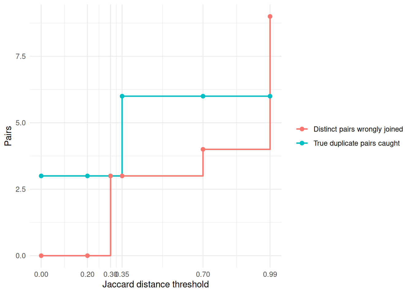
For this constructed set, 0.2917 is smaller than 0.32. The distractor is closer to the source than the paraphrase is. Because those two distances are ordered that way, no threshold on these pairs can catch the paraphrase without also joining the distractor. The sweep confirms that threshold choice trades one error against another here; it is not a general law of deduplication.
Deduplication at scale
The expand_grid() step used here builds an all-pairs combination, which mathematically scales at \(O(N^2)\). Pairwise comparisons work for a tiny teaching set, but mathematically collapse in production. For real-world datasets, an all-pairs Jaccard distance calculation is too slow and requires too much memory.
Production systems bypass this \(O(N^2)\) scaling boundary by using Locality Sensitive Hashing (LSH) and MinHash over shingled text. R packages like textreuse (or Python’s datasketch) implement these algorithms to group near-duplicates across millions of documents without comparing every pair.
What to remember
- Duplicate documents can inflate counts and leak between training and evaluation.
- Exact hashes catch only byte-for-byte repeats.
- Normalized hashes catch some formatting differences and erase formatting facts.
- Character-trigram Jaccard distance measures surface overlap, not preserved meaning.
- Near-duplicate thresholds trade missed duplicates against wrongly joined records in this set.
- The right threshold depends on which error costs more for the project.
Exact repeats can be removed automatically; near matches belong in review before any training or evaluation split. The threshold sweep is a warning label on this constructed set, not a universal setting for Riverton documents.