library(readr)
library(dplyr)
library(tibble)
library(tidyr)
library(purrr)
library(stringr)
library(ggplot2)
library(tidymodels)
library(textrecipes)
library(glmnet)
library(digest)

inbox_path <- "data/riverton/riverton-inbox.csv"
inbox <- read_csv(
  inbox_path,
  na = character(),
  col_types = cols(
    message_id = col_character(),
    text = col_character(),
    is_spam = col_logical(),
    intent = col_character(),
    author_note = col_character()
  )
)

inbox_metadata <- read_csv(
  "data/riverton/riverton-inbox-metadata.csv",
  na = character(),
  col_types = cols(
    artifact = col_character(),
    description = col_character(),
    source = col_character(),
    license = col_character(),
    created_on = col_character(),
    purpose = col_character(),
    rows = col_integer(),
    spam_class_counts = col_character(),
    intent_class_counts = col_character(),
    fingerprint = col_character()
  )
)

spam_counts <- inbox |>
  count(is_spam, name = "messages") |>
  mutate(class = if_else(is_spam, "job scam", "genuine message"))

inbox_hash <- digest(
  paste(read_lines(inbox_path), collapse = "\n"),
  algo = "sha256",
  serialize = FALSE
)Catching scam messages
Read a spam rule, train a small filter, and choose which mistake costs more
classification
spam detection
workforce research
Learn how spam detection turns text into decisions while keeping false alarms and missed scams separate.
Maya opens the Riverton Workforce Lab inbox before the morning appointments. Most messages ask ordinary questions about applications, passwords, and classes. Mixed into the same list are offers that ask jobseekers to send money.
If the Lab blocks too much, a real request can disappear. If it blocks too little, a scam can reach someone who is looking for work. A spam filter is a text classifier, a tool that assigns a label to a piece of writing.
Note
The Riverton Workforce Lab, its job board, and its training flyer are fictional and were created for teaching.
A dataset written by the same person who writes the classifier cannot measure whether the method works. This invented inbox checks that the code runs and makes the trade-off visible; it does not estimate performance for real spam filters.
TipWhat you will learn
By the end of this lesson, you will be able to:
- read a transparent spam rule;
- train a small text classifier;
- compare the rule and model where they disagree;
- read a confusion matrix; and
- explain how a decision threshold trades false alarms against missed scams.
Load the invented inbox
The inbox file was generated once by data-raw/build-riverton-inbox.R and then committed. The lesson reads that file; it does not write examples while the page renders. readr opens the CSV files, dplyr and tidyr shape tables, stringr reads patterns, ggplot2 draws the chart, tidymodels fits the classifier, textrecipes turns words into features, glmnet fits the model, and digest checks the file.
| Recorded class | Messages |
|---|---|
| genuine message | 44 |
| job scam | 16 |
The file has 60 invented messages: 44 genuine messages and 16 job scams. Those counts describe the fixture only. They do not say how much scam traffic reaches a workforce office.
Hand-written fixtures can fail before any model runs. The classes may separate on grammar rather than on the intended idea. A superficial feature is a cue such as punctuation or pronoun use that can predict a label without reading the substance of the message. The check below tests a bad shortcut: mark a message as spam when it has no first-person pronoun and does not end with a question mark.
first_person_pattern <- regex(
  "\\b(I|I'm|I’ve|I’d|I’ll|me|my|mine|we|we're|we’ve|us|our|ours)\\b",
  ignore_case = TRUE
)

surface_rule <- inbox |>
  mutate(
    first_person_pronoun = str_detect(text, first_person_pattern),
    terminal_question_mark = str_detect(text, "\\?\\s*$"),
    surface_spam = !first_person_pronoun & !terminal_question_mark,
    truth = factor(if_else(is_spam, "spam", "genuine"), levels = c("spam", "genuine")),
    estimate = factor(
      if_else(surface_spam, "spam", "genuine"),
      levels = c("spam", "genuine")
    )
  )

surface_confusion <- yardstick::conf_mat(
  surface_rule,
  truth = truth,
  estimate = estimate
)
surface_matrix <- as.matrix(surface_confusion$table)

surface_scores <- tibble(
  shortcut = "No first-person pronoun and no terminal question mark",
  accuracy = yardstick::accuracy(surface_rule, truth = truth, estimate = estimate) |>
    pull(.estimate),
  scam_recall = yardstick::sens(
    surface_rule,
    truth = truth,
    estimate = estimate,
    event_level = "first"
  ) |>
    pull(.estimate),
  genuine_recall = yardstick::spec(
    surface_rule,
    truth = truth,
    estimate = estimate,
    event_level = "first"
  ) |>
    pull(.estimate)
)| Shortcut | Accuracy | Scam recall | Genuine recall |
|---|---|---|---|
| No first-person pronoun and no terminal question mark | 0.6667 | 0.3125 | 0.7955 |
This shortcut scores 0.6667 accuracy and 0.3125 scam recall. That weak result is the point. When you write examples yourself, the two classes can separate on a pattern you did not mean to teach. The first check on any hand-built dataset is whether a stupid feature already solves it.
One shortcut is not the whole audit, so the next chunk sweeps several. For each feature it tries both orientations, marking a message as a scam when the feature is present and again when it is absent, and keeps whichever scores better. That is deliberately generous to the shortcut, because the question is whether any cheap cue could substitute for reading.
superficial_features <- inbox |>
  transmute(
    is_spam,
    `first-person pronoun` = str_detect(text, first_person_pattern),
    `ends with a question mark` = str_detect(text, "\\?\\s*$"),
    `longer than the median` = str_count(text, "\\S+") >= median(str_count(text, "\\S+")),
    `exclamation mark` = str_detect(text, "!"),
    `contains a digit` = str_detect(text, "[0-9]")
  ) |>
  pivot_longer(-is_spam, names_to = "feature", values_to = "present")

shortcut_sweep <- superficial_features |>
  reframe(
    spam_when_feature_is = c("present", "absent"),
    accuracy = c(
      mean(present == is_spam),
      mean(present != is_spam)
    ),
    scam_recall = c(
      mean(present[is_spam]),
      mean(!present[is_spam])
    ),
    .by = feature
  ) |>
  arrange(feature, desc(accuracy), desc(scam_recall)) |>
  slice_head(n = 1, by = feature) |>
  arrange(desc(accuracy), feature)

shortcut_display <- bind_rows(
  shortcut_sweep,
  tibble(
    feature = "always genuine baseline",
    spam_when_feature_is = "never",
    accuracy = mean(!inbox$is_spam),
    scam_recall = 0
  )
) |>
  arrange(desc(accuracy), feature)

length_feature_counts <- superficial_features |>
  filter(feature == "longer than the median") |>
  summarise(
    scams_above_median = sum(present & is_spam),
    genuine_above_median = sum(present & !is_spam)
)| Superficial feature | Predict spam when feature is | Accuracy | Scam recall |
|---|---|---|---|
| exclamation mark | present | 0.7667 | 0.1250 |
| always genuine baseline | never | 0.7333 | 0.0000 |
| contains a digit | present | 0.7333 | 0.1250 |
| first-person pronoun | absent | 0.6000 | 0.3125 |
| longer than the median | present | 0.5833 | 0.8125 |
| ends with a question mark | present | 0.5167 | 0.1875 |
No cue improves accuracy much beyond always predicting genuine. Exclamation marks improve accuracy by two messages, but catch only 2 of 16 scams. The digit cue exactly matches the 0.7333 majority baseline. Message length exposes another fixture artifact: 13 of 16 scams, but also 22 of 44 genuine messages, are longer than the median. That cue catches many scams while producing too many false alarms to classify well. These are diagnostics of how the hand-written file was made, not evidence that any cue will transfer. The way to find out is to test text that did not shape the examples or the rule.
The build script for this file recomputes the orientation-preserving sweep before writing the CSV and refuses to write if any single feature reaches 0.80 accuracy or 0.95 scam recall.
Start with a rule a person can read
A rule-based spam filter searches for known warning signs. This one marks a message when it mentions fees, gift cards, crypto payments, bank details, guaranteed placement, deposits, or similar language. The rule is easy to inspect, which also means it is easy for a scammer to route around.
spam_terms <- c(
  "fee", "payment", "gift card", "gift cards", "crypto",
  "wire transfer", "deposit", "bank", "card number",
  "guarantee", "guaranteed", "starter kit", "activation fee",
  "Social Security", "secret shopper", "premium number",
  "pay now", "\\$[0-9]+"
)

spam_pattern <- regex(
  paste(spam_terms, collapse = "|"),
  ignore_case = TRUE
)

term_hits <- tibble(term = spam_terms) |>
  mutate(
    messages_matched = map_int(
      term,
      \(term_text) sum(str_detect(inbox$text, regex(term_text, ignore_case = TRUE)))
    )
  )

rule_results <- inbox |>
  mutate(
    truth = factor(
      if_else(is_spam, "spam", "genuine"),
      levels = c("spam", "genuine")
    ),
    estimate = factor(
      if_else(str_detect(text, spam_pattern), "spam", "genuine"),
      levels = c("spam", "genuine")
    )
  )

rule_confusion <- yardstick::conf_mat(
  rule_results,
  truth = truth,
  estimate = estimate
)

rule_matrix <- as.matrix(rule_confusion$table)| Rule prediction | Recorded label | Messages |
|---|---|---|
| spam | spam | 14 |
| genuine | spam | 2 |
| spam | genuine | 2 |
| genuine | genuine | 42 |
The rule marks 14 of the 16 invented scams and also blocks two genuine messages. It misses two scams. In this fixture, the easy cases are the ones that say fee, deposit, or crypto plainly.
The word list was written after reading these messages. Eleven of its 18 terms match exactly one message, so the full 60-row table is a lookup table scored on the same rows that shaped it. The two blocked genuine messages were written with scam vocabulary on purpose to show that a readable rule can fail on reports about scams. The comparison below applies both methods to the same 19 rows, but that does not make the rule out-of-sample: its terms were chosen after reading all 60 messages, including those 19.
Train a small filter
A trained model learns word weights from labelled examples. The seed for the train-test split is 4801, and the seed before fitting is 4802. The split is stratified, meaning each side keeps both recorded classes.
set.seed(4801)
spam_data <- inbox |>
  mutate(
    spam_label = factor(
      if_else(is_spam, "spam", "genuine"),
      levels = c("spam", "genuine")
    )
  )

spam_split <- initial_split(
  spam_data,
  prop = 0.7,
  strata = spam_label
)
spam_train <- training(spam_split)
spam_test <- testing(spam_split)

spam_recipe <- recipe(spam_label ~ text, data = spam_train) |>
  step_tokenize(text) |>
  step_tokenfilter(text, max_tokens = 80) |>
  step_tfidf(text)

spam_model <- logistic_reg(penalty = 0.01, mixture = 1) |>
  set_engine("glmnet") |>
  set_mode("classification")

set.seed(4802)
spam_fit <- workflow() |>
  add_recipe(spam_recipe) |>
  add_model(spam_model) |>
  fit(data = spam_train)

probability_column <- predict(spam_fit, spam_test, type = "prob") |>
  names() |>
  keep(\(column) str_detect(column, "spam$"))

spam_scored <- spam_test |>
  select(message_id, text, is_spam, spam_label) |>
  bind_cols(predict(spam_fit, spam_test, type = "prob")) |>
  mutate(
    spam_probability = .data[[probability_column]],
    model_spam = spam_probability >= 0.5,
    rule_spam = str_detect(text, spam_pattern),
    model_label = factor(
      if_else(model_spam, "spam", "genuine"),
      levels = c("spam", "genuine")
    )
  )

model_confusion <- yardstick::conf_mat(
  spam_scored,
  truth = spam_label,
  estimate = model_label
)
model_matrix <- as.matrix(model_confusion$table)

test_rule_confusion <- yardstick::conf_mat(
  spam_scored |>
    mutate(
      rule_label = factor(
        if_else(rule_spam, "spam", "genuine"),
        levels = c("spam", "genuine")
      )
    ),
  truth = spam_label,
  estimate = rule_label
)
test_rule_matrix <- as.matrix(test_rule_confusion$table)

test_comparison <- tibble(
  method = c("Readable rule", "Trained model", "Always genuine"),
  correct = c(
    sum(spam_scored$rule_spam == spam_scored$is_spam),
    sum(spam_scored$model_spam == spam_scored$is_spam),
    sum(!spam_scored$is_spam)
  ),
  rows = nrow(spam_scored),
  accuracy = correct / rows,
  evidence_status = c(
    "in-sample: terms came from all 60 messages",
    "out-of-sample for the fitted model",
    "not fitted"
  )
)| Rule prediction | Recorded label | Messages |
|---|---|---|
| spam | spam | 3 |
| genuine | spam | 2 |
| spam | genuine | 1 |
| genuine | genuine | 13 |
| Model prediction | Recorded label | Messages |
|---|---|---|
| spam | spam | 3 |
| genuine | spam | 2 |
| spam | genuine | 3 |
| genuine | genuine | 11 |
| Method | Correct | Rows | Accuracy | Evidence status |
|---|---|---|---|---|
| Readable rule | 16 | 19 | 0.8421 | in-sample: terms came from all 60 messages |
| Trained model | 14 | 19 | 0.7368 | out-of-sample for the fitted model |
| Always genuine | 14 | 19 | 0.7368 | not fitted |
On the same 19 rows, the rule labels 3 of the 5 invented scams as spam and blocks one genuine message. Its 0.8421 accuracy is in-sample because the terms were written after reading all 60 messages. The model also catches 3 scams, but blocks three genuine messages. Its out-of-sample accuracy is 0.7368, exactly the always-genuine baseline on this split. The rule and model therefore cannot be ranked as held-out competitors. The table does show why a score needs a baseline: without one, a fitted model can look informative while matching a trivial rule.
Look at the disagreements
The rule and the model do not mark the same messages. Disagreements are useful because a person can inspect a short list and ask which tool failed in a way that matters.
disagreements <- spam_scored |>
  filter(rule_spam != model_spam) |>
  arrange(message_id) |>
  mutate(
    recorded_label = if_else(is_spam, "spam", "genuine"),
    spam_probability = round(spam_probability, 3)
  ) |>
  select(
    message_id,
    recorded_label,
    spam_probability,
    rule_spam,
    model_spam,
    text
)| Message | Recorded label | Model spam score | Rule says spam | Model says spam | Text |
|---|---|---|---|---|---|
| M004 | genuine | 0.972 | FALSE | TRUE | Please confirm that my documents for the youth internship reached your office. |
| M030 | genuine | 0.869 | FALSE | TRUE | Can I apply to the data support certificate with a GED? |
| M034 | genuine | 0.010 | TRUE | FALSE | A listing says paid training, but the attachment asks for my bank password. |
| M046 | genuine | 0.998 | FALSE | TRUE | Could you call with bus directions to the skills centre? |
The message about documents reaching the office looks genuine to the recorded label but receives a high model score. The message about a bank password is genuine because it reports a suspicious listing, yet the rule catches the word bank. The two callback and eligibility messages show the model’s own false alarms. Those are different kinds of errors.
Move the cut point
The model produces a score between 0 and 1. The cut point turns that score into a decision. A lower cut point catches more possible scams and risks blocking more genuine messages. A higher cut point does the reverse.
This curve uses the same 19 rows as the model table. Choosing a cut point from the curve and then reporting its errors on these rows would spend the test set twice. A deployed threshold should be chosen on separate calibration data before the final test.
threshold_table <- tibble(threshold = seq(0.05, 0.95, by = 0.05)) |>
  mutate(
    results = map(threshold, \(cut_point) {
      spam_scored |>
        summarise(
          genuine_blocked = sum(spam_probability >= cut_point & !is_spam),
          scams_missed = sum(spam_probability < cut_point & is_spam),
          sent_to_review = sum(spam_probability >= cut_point),
          .groups = "drop"
        )
    })
  ) |>
unnest(results)| Spam score cut point | Genuine messages blocked | Scams missed | Messages sent to spam review |
|---|---|---|---|
| 0.05 | 4 | 1 | 8 |
| 0.10 | 3 | 1 | 7 |
| 0.15 | 3 | 1 | 7 |
| 0.20 | 3 | 1 | 7 |
| 0.25 | 3 | 1 | 7 |
| 0.30 | 3 | 2 | 6 |
| 0.35 | 3 | 2 | 6 |
| 0.40 | 3 | 2 | 6 |
| 0.45 | 3 | 2 | 6 |
| 0.50 | 3 | 2 | 6 |
| 0.55 | 3 | 2 | 6 |
| 0.60 | 3 | 2 | 6 |
| 0.65 | 3 | 2 | 6 |
| 0.70 | 3 | 2 | 6 |
| 0.75 | 3 | 2 | 6 |
| 0.80 | 3 | 2 | 6 |
| 0.85 | 3 | 2 | 6 |
| 0.90 | 2 | 2 | 5 |
| 0.95 | 2 | 3 | 4 |
Show the plotting code
source("R/lesson-figures.R")

threshold_plot <- threshold_table |>
  select(threshold, genuine_blocked, scams_missed) |>
  pivot_longer(
    cols = c(genuine_blocked, scams_missed),
    names_to = "error_type",
    values_to = "messages"
  ) |>
  mutate(
    error_type = recode(
      error_type,
      genuine_blocked = "genuine messages blocked",
      scams_missed = "scams missed"
    )
  )

error_colours <- c(
  "genuine messages blocked" = lesson_colours[["accent"]],
  "scams missed" = lesson_colours[["contrast"]]
)
error_label_colours <- c(
  "genuine messages blocked" = lesson_text_colours[["accent"]],
  "scams missed" = lesson_text_colours[["contrast"]]
)

ggplot(threshold_plot, aes(x = threshold, y = messages, colour = error_type)) +
  geom_step(aes(linetype = error_type), linewidth = 0.9, direction = "hv") +
  geom_point(size = 2) +
  geom_text(
    data = \(d) filter(d, threshold == max(threshold)),
    aes(label = error_type, colour = I(error_label_colours[error_type])),
    hjust = 0,
    nudge_x = 0.03,
    family = lesson_font,
    size = 10,
    size.unit = "pt"
  ) +
  scale_colour_manual(values = error_colours, guide = "none") +
  scale_linetype_manual(
    values = c("genuine messages blocked" = "solid", "scams missed" = "22"),
    guide = "none"
  ) +
  scale_x_continuous(
    breaks = seq(0.1, 0.9, by = 0.2),
    expand = expansion(mult = c(0.02, 0.38))
  ) +
  scale_y_continuous(breaks = 0:4, limits = c(0, 4)) +
  labs(
    title = "Raising the cut point trades false alarms for missed scams",
    subtitle = "Errors on the 19 invented test messages at each spam-score cut point",
    x = "Spam score cut point",
    y = "Messages"
  ) +
  theme_lesson(grid = "y")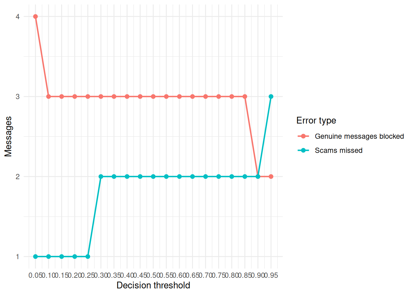
For this invented split, thresholds from 0.30 through 0.85 have the same error counts: three genuine messages blocked and two scams missed. Only the low and high ends move the counts. That is a number about this fixture, not about the world. A company inbox might prefer to block anything suspicious. A workforce inbox serving jobseekers may need a review queue because deleting a genuine posting can cost someone an opportunity, while letting a scam through can cost money or personal information.
Real spam also adapts. A static test set cannot measure what happens after senders learn the filter’s habits and change their wording.
What to remember
- Spam detection is text classification with unequal errors.
- A readable rule helps inspection, but it is brittle.
- A trained model still needs a human-chosen threshold.
- Every score needs a baseline and a named test set.
- The Riverton inbox proves only that the lesson code runs on an invented file.