library(dplyr)
library(ggplot2)
library(purrr)
library(stringr)
library(tibble)
library(tidyr)

source("R/lesson-figures.R")

program_entries <- tribble(
  ~entry_id, ~entry_date, ~entry_text,
  "R01", "2026-02-20",
  "The spring outreach window will run this spring.",
  "R02", "2026-03-03",
  "The orientation was held on March 2, and registration closes on March 15.",
  "R03", "2026-08-28",
  "The 12-week course starts on September 14.",
  "R04", "2026-09-20",
  "The reminder says the applicant check-in happened last Monday.",
  "R05", "2026-10-05",
  "The pilot lasted six weeks.",
  "R06", "2026-10-10",
  "The October review meeting is planned for October 22.",
  "R07", "2026-11-01",
  "The November report covers work completed in September."
) |>
mutate(entry_date = as.Date(entry_date))Putting events on a timeline
Keep document dates, event dates, and uncertain durations apart
information visualization
timelines
temporal parsing
Learn how to draw a small event timeline without turning coarse or missing dates into false points.
The pilot lasted six weeks looks ready for a timeline until Nadia asks when the six weeks began. Other entries report a day, a month, or a season.
Events on a timeline means placing event records on a time scale only as precisely as the text allows. A day can be a point. A month, season, or course length needs an interval. A duration with no start date stays off the time scale.
This lesson uses a small constructed log so the dates can be checked by eye. It builds on the temporal parsing lesson, which explains reference dates for phrases such as “next Friday.”
Note
The Riverton program log in this lesson is a constructed teaching example about an invented service desk; the entries and normalized dates were written by this lesson’s author.
TipWhat you will learn
This lesson shows how to:
- keep the date of a note separate from the date of the event it mentions;
- resolve relative dates from each note’s own date;
- draw seasons, months, and course lengths as intervals;
- mark planned and reported events without relying on colour alone;
- show an undated event without guessing its position; and
- compare the order of the notes with the order of the events.
Build a small event log
An entry date is the date the note was written. It is the anchor for relative language, not automatically the date of the event. The entry_id stays with every row so each mark on the timeline can be traced back to its source sentence.
| Entry ID | Entry date | Constructed log entry |
|---|---|---|
| R01 | 2026-02-20 | The spring outreach window will run this spring. |
| R02 | 2026-03-03 | The orientation was held on March 2, and registration closes on March 15. |
| R03 | 2026-08-28 | The 12-week course starts on September 14. |
| R04 | 2026-09-20 | The reminder says the applicant check-in happened last Monday. |
| R05 | 2026-10-05 | The pilot lasted six weeks. |
| R06 | 2026-10-10 | The October review meeting is planned for October 22. |
| R07 | 2026-11-01 | The November report covers work completed in September. |
The second entry has two events and two dates. The orientation belongs to March 2. The registration closing belongs to March 15. Reading only the nearest date would fail on many real sentences, so here the attachment is recorded by hand.
Normalize only what the text supports
The table of events below names each event’s trigger, its time expression, and the rule used to compute its dates. The season rule is a local convention: this page uses Northern Hemisphere meteorological seasons, so spring runs from March 1 through May 31.
season_bounds <- tribble(
  ~season, ~start_month, ~start_day, ~end_month, ~end_day,
  "spring", 3L, 1L, 5L, 31L,
  "summer", 6L, 1L, 8L, 31L,
  "autumn", 9L, 1L, 11L, 30L,
  "winter", 12L, 1L, 2L, 28L
)

event_plan <- tribble(
  ~event_id, ~entry_id, ~trigger, ~time_text, ~granularity, ~status, ~rule,
  "EV01", "R01", "outreach window", "this spring", "season", "planned",
  "entry-year spring",
  "EV02", "R02", "orientation held", "March 2", "day", "reported",
  "entry-year month day",
  "EV03", "R02", "registration closes", "March 15", "day", "planned",
  "entry-year month day",
  "EV04", "R03", "12-week course", "September 14 for 12 weeks", "duration",
  "planned", "entry-year month day plus weeks",
  "EV05", "R04", "applicant check-in", "last Monday", "day", "reported",
  "previous weekday from entry date",
  "EV06", "R05", "pilot lasted", "six weeks", "duration", "reported",
  "duration without start",
  "EV07", "R06", "review meeting", "October 22", "day", "planned",
  "entry-year month day",
  "EV08", "R07", "September work", "September", "month", "reported",
  "entry-year month"
)

make_date <- function(year, month, day) {
  as.Date(sprintf("%04d-%02d-%02d", year, month, day))
}

parse_month_day <- function(entry_date, time_text) {
  parts <- str_match(time_text, "\\b([A-Z][a-z]+)\\s+(\\d{1,2})\\b")
  make_date(
    as.integer(format(entry_date, "%Y")),
    match(parts[, 2], month.name),
    as.integer(parts[, 3])
  )
}

parse_month_interval <- function(entry_date, time_text) {
  month_number <- match(time_text, month.name)
  start <- make_date(as.integer(format(entry_date, "%Y")), month_number, 1L)
  end <- seq(start, by = "1 month", length.out = 2L)[2] - 1L
  list(start = start, end = end)
}

previous_weekday <- function(entry_date, weekday) {
  weekday_names <- c(
    "Sunday", "Monday", "Tuesday", "Wednesday",
    "Thursday", "Friday", "Saturday"
  )
  current_day <- as.POSIXlt(entry_date)$wday + 1L
  target_day <- match(weekday, weekday_names)
  days_back <- (current_day - target_day) %% 7L
  if (days_back == 0L) {
    days_back <- 7L
  }
  entry_date - days_back
}

placed_interval <- function(start, end) {
  list(start = start, end = end, placed = TRUE, reason_unplaced = NA_character_)
}

normalize_event <- function(rule, entry_date, time_text) {
  entry_year <- as.integer(format(entry_date, "%Y"))

  if (rule == "entry-year spring") {
    bounds <- season_bounds |>
      filter(season == "spring")
    return(placed_interval(
      make_date(entry_year, bounds$start_month, bounds$start_day),
      make_date(entry_year, bounds$end_month, bounds$end_day)
    ))
  }

  if (rule == "entry-year month day") {
    day <- parse_month_day(entry_date, time_text)
    return(placed_interval(day, day))
  }

  if (rule == "entry-year month day plus weeks") {
    start <- parse_month_day(entry_date, time_text)
    return(placed_interval(start, start + 12L * 7L - 1L))
  }

  if (rule == "previous weekday from entry date") {
    day <- previous_weekday(entry_date, "Monday")
    return(placed_interval(day, day))
  }

  if (rule == "entry-year month") {
    interval <- parse_month_interval(entry_date, time_text)
    return(placed_interval(interval$start, interval$end))
  }

  list(
    start = as.Date(NA),
    end = as.Date(NA),
    placed = FALSE,
    reason_unplaced = "duration has no start date"
  )
}

event_rows <- event_plan |>
  left_join(program_entries, by = join_by(entry_id)) |>
  mutate(
    normalized = pmap(list(rule, entry_date, time_text), normalize_event),
    start = as.Date(map_chr(normalized, \(item) as.character(item$start))),
    end = as.Date(map_chr(normalized, \(item) as.character(item$end))),
    placed = map_lgl(normalized, "placed"),
    reason_unplaced = map_chr(normalized, "reason_unplaced"),
    narrative_order = match(entry_id, program_entries$entry_id)
  ) |>
  select(
    event_id, entry_id, narrative_order, entry_date, trigger, time_text,
    granularity, status, rule, start, end, placed, reason_unplaced
)| Event ID | Entry ID | Entry date | Event trigger | Time text | Granularity | Status | Rule | Start | End | Reason not placed |
|---|---|---|---|---|---|---|---|---|---|---|
| EV01 | R01 | 2026-02-20 | outreach window | this spring | season | planned | entry-year spring | 2026-03-01 | 2026-05-31 | NA |
| EV02 | R02 | 2026-03-03 | orientation held | March 2 | day | reported | entry-year month day | 2026-03-02 | 2026-03-02 | NA |
| EV03 | R02 | 2026-03-03 | registration closes | March 15 | day | planned | entry-year month day | 2026-03-15 | 2026-03-15 | NA |
| EV04 | R03 | 2026-08-28 | 12-week course | September 14 for 12 weeks | duration | planned | entry-year month day plus weeks | 2026-09-14 | 2026-12-06 | NA |
| EV05 | R04 | 2026-09-20 | applicant check-in | last Monday | day | reported | previous weekday from entry date | 2026-09-14 | 2026-09-14 | NA |
| EV06 | R05 | 2026-10-05 | pilot lasted | six weeks | duration | reported | duration without start | NA | NA | duration has no start date |
| EV07 | R06 | 2026-10-10 | review meeting | October 22 | day | planned | entry-year month day | 2026-10-22 | 2026-10-22 | NA |
| EV08 | R07 | 2026-11-01 | September work | September | month | reported | entry-year month | 2026-09-01 | 2026-09-30 | NA |
Seven events receive dates. One duration does not. The start and end columns make the difference visible: a day has the same start and end. The spring and September intervals cover only the season or month named in the entry; only the 12-week course interval is a known duration.
The “pilot lasted six weeks” row gives a length but no position. Nadia keeps it in the table, and the timeline gives it a row with no mark rather than a guessed one.
Draw the notes and the events together
The timeline below gives every event its own row, sorted by when the event happened, with the undated pilot last. Each row shows two dates. The grey diamond is the day the note was written, and the dotted line leads from it to the event the note describes. Days are points; seasons, months, and the course length are bars.
Status has two cues so it does not depend on colour: planned events are hollow points or dashed bars, and reported events are filled points or solid bars. In this constructed log, every reported event comes before its note and every planned event after it, so the dotted lines of reported events point back in time and those of planned events point forward. Real notes can report ongoing work or record a plan after the fact, so direction is a check to run, not a rule.
status_colours <- c(
  planned = lesson_colours[["accent"]],
  reported = lesson_colours[["contrast"]]
)

timeline_rows <- event_rows |>
  arrange(!placed, start, end, event_id) |>
  mutate(
    row_label = str_c(str_to_sentence(trigger), " (", entry_id, ")"),
    row_label = factor(row_label, levels = rev(row_label)),
    # The dotted line runs from the note to the nearest edge of the event.
    link_end = case_when(
      !placed ~ as.Date(NA),
      start > entry_date ~ start,
      end < entry_date ~ end,
      TRUE ~ entry_date
    )
  )

timeline_plot <- ggplot(timeline_rows, aes(y = row_label)) +
  geom_segment(
    data = \(d) filter(d, placed),
    aes(x = entry_date, xend = link_end),
    colour = lesson_colours[["muted"]],
    linewidth = 0.5,
    linetype = "dotted"
  ) +
  geom_segment(
    data = \(d) filter(d, placed, granularity != "day"),
    aes(x = start, xend = end, colour = status, linetype = status),
    linewidth = 3.2
  ) +
  geom_point(
    data = \(d) filter(d, placed, granularity == "day"),
    aes(x = start, colour = status, shape = status),
    size = 3.4,
    stroke = 1.3,
    fill = lesson_colours[["paper"]]
  ) +
  geom_point(
    aes(x = entry_date),
    shape = 23,
    size = 2.6,
    fill = lesson_colours[["muted"]],
    colour = lesson_colours[["paper"]]
  ) +
  geom_text(
    data = \(d) filter(d, !placed),
    aes(x = entry_date, label = "no start date, so no mark"),
    hjust = 1,
    nudge_x = -8,
    family = lesson_font,
    size = 9.5,
    size.unit = "pt",
    colour = lesson_colours[["muted"]]
  ) +
  scale_y_discrete(drop = FALSE) +
  scale_colour_manual(values = status_colours) +
  scale_linetype_manual(values = c(planned = "22", reported = "solid")) +
  scale_shape_manual(values = c(planned = 21, reported = 19)) +
  scale_x_date(
    date_breaks = "1 month",
    date_labels = "%b",
    limits = as.Date(c("2026-01-15", "2026-12-20")),
    expand = expansion(mult = 0)
  ) +
  labs(
    title = "An event's date is not the date of the note that mentions it",
    subtitle = str_c(
      "Constructed Riverton log, 2026. Grey diamonds are entry dates; ",
      "dotted lines lead to ",
      lesson_key("planned", lesson_text_colours[["accent"]]),
      " and ",
      lesson_key("reported", lesson_text_colours[["contrast"]]),
      " events."
    ),
    x = NULL,
    y = NULL
  ) +
  theme_lesson(grid = "x") +
  theme(legend.position = "none")

timeline_plot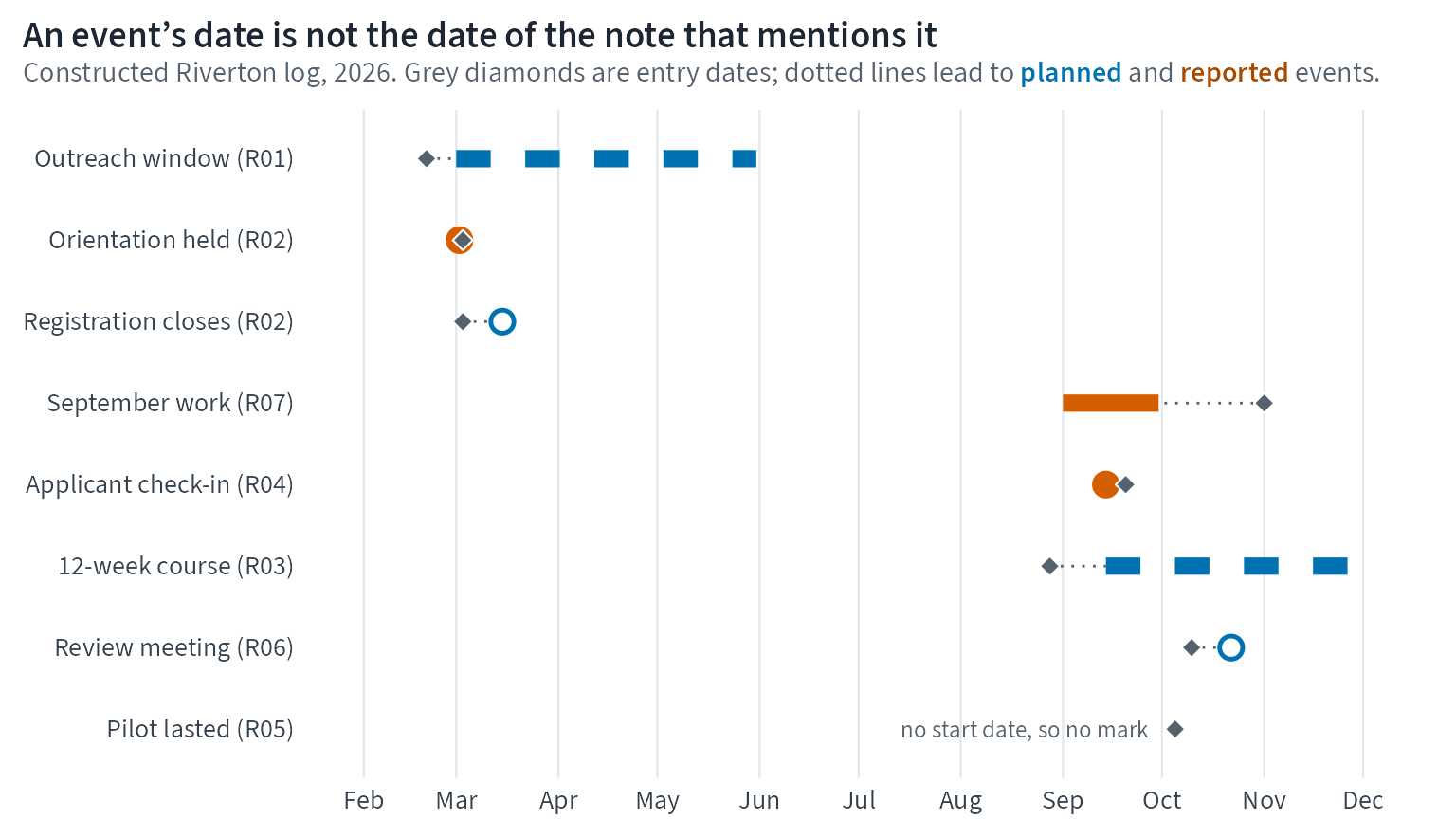
The rows follow event order, but each label also names its source entry, which shows the order of the notes. The November report is entry R07, yet its September work sits above the October review meeting, and its dotted line runs back from November. That difference is why a timeline should not treat the order of the notes as time.
The event table is the long description for the figure. It gives the exact dates, status, and entry ID for each mark.
timeline_long_description <- timeline_rows |>
  mutate(event_order = if_else(placed, row_number(), NA_integer_)) |>
  select(
    event_order, narrative_order, event_id, entry_id, entry_date, trigger,
    time_text, granularity, status, start, end
)| Event order | Narrative order | Event ID | Entry ID | Entry date | Event trigger | Time text | Granularity | Status | Start | End |
|---|---|---|---|---|---|---|---|---|---|---|
| 1 | 1 | EV01 | R01 | 2026-02-20 | outreach window | this spring | season | planned | 2026-03-01 | 2026-05-31 |
| 2 | 2 | EV02 | R02 | 2026-03-03 | orientation held | March 2 | day | reported | 2026-03-02 | 2026-03-02 |
| 3 | 2 | EV03 | R02 | 2026-03-03 | registration closes | March 15 | day | planned | 2026-03-15 | 2026-03-15 |
| 4 | 7 | EV08 | R07 | 2026-11-01 | September work | September | month | reported | 2026-09-01 | 2026-09-30 |
| 5 | 4 | EV05 | R04 | 2026-09-20 | applicant check-in | last Monday | day | reported | 2026-09-14 | 2026-09-14 |
| 6 | 3 | EV04 | R03 | 2026-08-28 | 12-week course | September 14 for 12 weeks | duration | planned | 2026-09-14 | 2026-12-06 |
| 7 | 6 | EV07 | R06 | 2026-10-10 | review meeting | October 22 | day | planned | 2026-10-22 | 2026-10-22 |
| NA | 5 | EV06 | R05 | 2026-10-05 | pilot lasted | six weeks | duration | reported | NA | NA |
How this differs from parsing one date
TimeML and related standards separate events, time expressions, and the document’s creation time. This page does the same thing in a small table. It does not train or evaluate a temporal parser, and the constructed normalizations are not independent labels.
A real-text case shows why the table matters. In the inaugural corpus, Lincoln’s 1865 phrase “four years ago” can be anchored only to a speech year if the source records no month or day. The output should keep that year-level granularity rather than inventing a day.
What to remember
- The entry date anchors relative phrases, but it is not the event date.
- A season or month is an interval under a stated convention.
- A day-level event can be a point; a coarser event should not be.
- Planned and reported events need a cue besides colour.
- A duration without a start date gets a row but no mark.
Nadia’s timeline is useful because it refuses one false mark. The six-week pilot is still visible, but it stays off the time scale until a start date appears.